Description
In the Functions tab, you can choose a distribution function and change other parameters affecting how grid point spacings vary along the length of the selected subconnector(s). The simple table at the top of this tab shows how many subconnectors are currently selected.
Note: When opening a Fidelity Pointwise project file that was saved using an older version of the software, you will be prompted to indicate whether to preserve the grid points locations or their distribution function. This information will be used in case the software cannot compute a distribution that matches exactly the grid points locations saved in the file using improved methods.
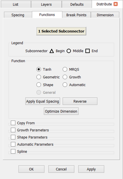
Function
The Function frame provides radio buttons for selecting the desired grid point distribution function. The available options are:
- Tanh: The default distribution function is the hyperbolic tangent (Ref. 38). If the spacing is unconstrained at both ends, grid points will be distributed uniformly using a simple uniform interpolation scheme. If the spacing is unconstrained at only one end, an alternative one-sided hyperbolic tangent distribution function is used. Hyperbolic tangent works very well for the majority of cases and for that reason it is the default distribution function.
- MRQS: The Monotonic Rational Quadratic Spline (MRQS) function (Ref. 1) can be applied to several subconnectors simultaneously. It forces a grid point to be fixed to a break point. At the same time, spacing continuity and spacing variation continuity will be applied automatically across the break point. This type is included for compatibility with existing Gridgen grids.
- Geometric: This is a one-sided distribution function. Only one spacing constraint on a subconnector can be set with this function type. Whichever spacing constraint was set last will be applied. If no spacing constraints are specified, the grid points will be distributed uniformly. Geometric progression works by distributing the grid points from the constrained end so the ratio of spacing between adjacent grid points is constant. Therefore, if tight clustering is specified at one end, the distance between successive points will increase monotonically towards the other end of the subconnector.
- Growth: This type allows you to modify a connector or subconnector to match the desired T-Rex parameters (refer to the T-Rex section for further information) such as the initial boundary layer spacing, growth rate, number of anisotropic layers, etc. It applies the geometric function to the boundary layer (“growth”) portion of a connector while the hyperbolic tangent function to the non-growth portion. It can be used as a one-sided function or two-sided. The one-sided growth is enabled by constraining the spacing on one end and setting its Growth Parameters to non-zero values. Likewise, the two-sided growth is enabled by constraining both spacings with their distribution parameters set to nonzero values. See more below on the Growth Parameters command frame. Selecting this function opens that frame automatically.
- Shape: This type allows you to enter values for the maximum deviation of the discrete connector from the segment shape and the maximum turning angle allowed between adjacent grid points along the connector. Note that unlike implementations of this feature in the Defaults panel and during connector dimensioning, the connector dimension is NOT changed when this feature is applied as a distribution function. This means that the deviation and turning angle limits you specify here will not be enforced exactly, but the general trend in grid point clustering will be applied. Furthermore, if you choose to maintain beginning and ending spacing constraints when applying this distribution function be aware that the level to which the limits will be enforced is seriously degraded. Use the Shape Parameters command frame (see below) to set the desired parameter values. Selecting this function opens that frame automatically.
- Automatic: The Automatic function attempts to create a size field from which to determine the distribution of grid points on a selected connector and implicitly its dimension as well. This function is governed by the attributes specified in the Automatic Parameters frame described below. Selecting this function will automatically open the parameters frame. The size field will depend on nearby or underlying database entities, as well as Sources. There is one exception to this set of size field influencers: when using boundary adaption in the Solve command, the block's size field will be applied, which can include grid entity influencers as well. If Automatic is the default distribution function, it will be applied at creation of new connectors. In all instances other than connector creation and block boundary adaption, it will be necessary to use the Optimize Dimension command to enforce or update the distribution. This command is available in this panel and also Grid toolbar.
- General: A general distribution results from other operations and cannot be set explicitly on any connector or subconnector. General distributions represent discrete point locations stored rather than points being located along a connector by a formula. These distributions will result from, for example, connectors being projected onto database surface entities or from connectors imported from a nonnative file format, such as Plot3D. This radio button choice is shown only for reference to indicate when such a distribution exists on a selected subconnector.
Tip: Use the Growth distribution function to produce a connector grid point distribution that matches a T-Rex anisotropic layer.
The Apply Equal Spacing command is a shortcut used to quickly unconstrain both ends of a subconnector by setting both values to zero. It also sets the distribution function back to the default: hyperbolic tangent.
The Reverse command is used to swap the constraint values from one end of a subconnector to the other while maintaining the original distribution function. Therefore, if a break point is dividing a connector into two subconnectors and both are selected in the Display window, Reverse will swap the constraint values on the ends of the first subconnector and also on the ends of the second subconnector.
In a nutshell, the Optimize Dimension command is used to change the dimension of the selected subconnector(s) in order to obtain the smoothest possible distribution of grid points. This can be accomplished in the following ways:
- Growth distribution function: When there is a discrepancy between the grid point spacing in the Middle region of the selected subconnector(s) (denoted by the ◯ symbol) and the grid point spacing of the final layer(s) as computed by the applied Growth distribution function (Begin and/or End), the Optimize Dimension command will add or remove grid points in order to produce the smoothest possible distribution.
- Tanh distribution function: When this distribution is applied to the selected subconnector(s), if one of the spacing constraints of the subconnector(s) has been specified by the user, the Optimize Dimension command will add or remove grid points in order to produce an equally spaced distribution. On the other hand, if both spacing constraints on the subconnector(s) have been defined by the user, the Optimize Dimension command will add or remove grid points to produce a smoothest possible distribution between the two specified spacing constraints.
- Automatic distribution function: When this distribution is applied to the selected subconnector(s), the Optimize Dimension command is used to enforce or update the distribution based on the defined size field parameters.
Copy From
The Copy From command becomes enabled when at least one subconnector is selected. Use the commands in this frame to copy the distribution of grid points from other subconnector(s) to the subconnector(s) currently selected. Opening this frame disables all other commands on the Functions tab.
Note that the selection of subconnectors can only be performed from the Display window; the List panel is not available to be used with the Copy From command. Once selected, the subconnectors are rendered in yellow with an arrow pointing to their end and representing their orientation. Furthermore, a color coded table lists the number of currently selected subconnectors to copy from and the total number of points they contain.
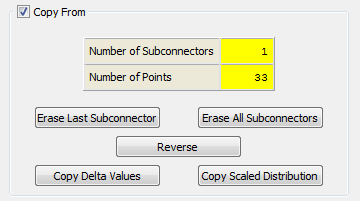
The Erase Last Subconnector command removes the most recently selected subconnector from the pending string to copy from. The Erase All Subconnectors command restarts the string selection. The Reverse command, reverses the orientation of the subconnector string.
The Copy Delta Values command completes the copy operation by enforcing the spacing constraints and function type of the pending subconnector(s) on the subconnector(s) currently selected for function change. This command is only available when a single subconnector is selected to copy from. On the other hand, the Copy Scaled Distribution command completes the copy operation by scaling the point distribution of the pending subconnector(s) by arc length to the subconnector(s) currently selected for function change.
Growth parameters
The Growth Parameters frame is closed by default. Once the Growth distribution Function is selected, the command frame opens automatically. The settings found in this frame are used in conjunction with the mentioned distribution function.
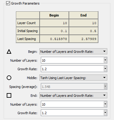
A growth distribution off the begin/end spacing constraint can be defined by one of the following methods: Number of Layers and Growth Rate, Total Height and Growth Rate, or Number of Layers and Total Height. Once this is selected from the Begin/End pull-down list, you can set the corresponding variables to non-zero values. As seen in the figure above, a two-sided growth distribution is created by setting the number of layers and growth rates for both ends of a connector (or subconnector).
Additionally, three options are available to control the Middle distribution, or the distribution of points outside of the T-Rex layers: Growth Until Specified Spacing, Tanh Using Last Layer Spacing, and Tanh Using Specified Spacing. Growth Until Specified Spacing continues the geometric growth of layers found inside the T-Rex layers until the spacing reaches a user specified value entered into the Spacing text field below the Middle pull-down. Tanh Using Last Layer Spacing (the default setting) will apply a hyperbolic tangent distribution in this region outside of the T-Rex layers with a spacing adjacent and equivalent to the last layer. Finally, Tanh Using Specified Spacing will also use hyperbolic tangent for the distribution but the spacing adjacent to the last T-Rex layer will be user specified.
If the user input requires a change in the dimension on the selected subconnector(s) to obtain a smooth distribution of grid points, click on Optimize Dimension to apply the optimal dimension to the selected connectors(s) based on the defined growth parameters.
Shape Parameters
The Shape Parameters frame is closed by default. Once this distribution Function is selected, the command frame opens automatically. The settings found in this frame are used in conjunction with the Shape distribution function (see above). Furthermore, they do not effectively change the dimension of the selected connectors.
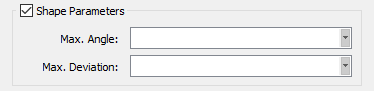
The Max. Angle parameter, lets you enter a maximum angular deviation in degrees. If the angle between the normal to a connector's line segment and the normal to the underlying database curve (or analytic curve defining the shape of the connector if not database constrained) at a grid point is larger than the specified angle, grid points on the connector being evaluated will be moved to attempt to satisfy the specified value.
On the other hand, the Max. Deviation parameter lets you specify a maximum chordal deviation between the discrete shape of the connector and the underlying database curve (or analytic curve defining the shape of the connector if not database constrained).
It is important to keep in mind that these parameters do not change the dimension of the selected connector. That is, existing points will be moved to attempt to satisfy the input turning angle constraint.
Automatic parameters
The Automatic Parameters frame is closed by default. Once this distribution Function is selected, the command frame opens automatically. The settings found in this frame are used in conjunction with the Automatic distribution function.
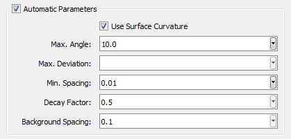
Note: All parameters set in the Automatic Parameters frame are stored as unique attributes of the connectors for which changes have been applied.
The Use Surface Curvature command, when checked on, allows a size field to be calculated from database and source entities in proximity of the selected subconnector(s). The influence of nearby database entities to the size field spacing is determined from their local curvature as enforced by the Max. Angle and Max. Deviation limits.
The Max. Angle parameter, lets you enter a maximum angular deviation in degrees. To understand how this parameter is used, let us consider an arbitrary sample point on a database curve or surface denoted point_A. Let us also consider all the "neighboring" sample points located on the same database curve or surface around point_A. Now imagine straight segments connecting our sample point point_A with each one of the "neighboring" sample points. If the angle between the normal to each one of such straight segments and the normal to the database curve or surface at point_A is larger than the specified Max. Angle value, the local point spacing around point_A will be decreased as necessary starting from the Background Spacing, if specified. Otherwise, a starting background spacing is determined from the entity extents.
Max. Deviation similarly specifies a maximum chordal deviation between the local discrete shape of the database between sample points and its analytic shape. Using the sample point_A and its "neighboring" sample points on the database curve or surface described above, if the maximum distance between the underlying database entity and each one of the straight segments connecting point_A to its neighboring sample points is larger than the specified Max. Deviation value, the local point spacing around point_A will be decreased as necessary.
The size field is also impacted by the Background Spacing and Decay Factor. These attributes will populate with the defaults from the Defaults panel. Background Spacing is a target baseline spacing to be applied in the absence of database entities or sources. Decay Factor varies from 0.0 to 1.0; a value of 0.0 indicates no influence beyond the boundary of the influence database entities, while a value of 1.0 indicates maximum influence. An additional limiter on the size field spacing, Min. Spacing, is a target minimum spacing to be used in the size field. Local values may vary below this setting, but will not fall significantly below the target.
If the Use Surface Curvature option is not checked, connector distribution will revert to only curvature along the arclength of the connector, as long as either Max. Angle or Max. Deviation are applied, in addition to any sources and Background Spacing. In the absence of Max. Angle or Max. Deviation limits, only sources and Background Spacing will be considered, as long as either sources are in proximity and shown (see Show/Hide), or if a Background Spacing has been specified. All of the Automatic function parameters can also be specified in the Defaults panel allowing quick and easy application of this function type during connector creation.
Spline
The Spline frame is also closed by default. Here you can change the Spline Variable from the default setting, Arclength.
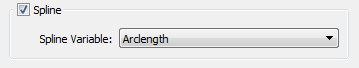
The Arclength setting forces grid points to be distributed based on arc length along the connector. Hence, a spacing constraint of 0.4 will make the distance between adjacent grid points at the end be 0.4. However, you may want to distribute grid points on the basis of only one of the coordinate components such as X, Y or Z instead of Arclength. If the spline variable is changed to X, for example, a spacing constraint of 0.4 will result in a grid point distribution such that the difference in X coordinate values of grid points will be 0.4.